Optimizing lookups on small string sets


Introduction
Since modern x86 architectures include several caching layers [1], it’s beneficial to understand how to best utilize them when it comes to designing data processing algorithms. Similarly to the ratio of today’s storage access latencies to main memory access latencies, which is about 1000:1 [2], access to modern x86 L1 cache is about 100 times faster [2] than accessing data in main memory. Also, just as with storage media, sequential access to data in main memory is faster than doing random accesses [3]. If we were to look at the layers from the CPU’s perspective, they behave just as progressively slower and bigger storage media. With this in mind, it makes sense to look past the storage/main memory boundary when designing modern data storage structures and algorithms. This is the core idea behind the ‘cache friendly’ term. As we’ve already developed a wide array of techniques to help working with slow(er) storage [4], we can reuse them here. Most of these techniques boil down to grouping data in some way and organizing these groups in some tree-like structures. The basic idea is to look at the time complexity through the lens of I/O access and prioritize it over computational complexity. We can look at a B+ tree structure as an example. With a fanout factor of k, accessing an element from n elements on the storage takes \(log_k(n)\) I/O operations to fetch it [5]. If the analogy between cache vs main memory and main memory vs storage holds, we can view time complexity through the lens of cache misses and prioritize that over computation complexity. The caveat here is that the scale on which we now operate is smaller and computational complexity, while second, is a close second to cache misses and must be taken into account.
Anyway, why am I telling you all of this? Well, I’m working on a database project [6]. It’s based on LSM trees [7]. In essence, with LSM trees, whenever new data comes in a new structure is created to hold it. When querying, queries are made on the existing structures and results are merged. Occasionally, existing structures are merged into a bigger one replacing them as a result. The data is never modified, only appended as is the case with logs. Supporting structures can be implemented in any number of ways but, as was already noted, common building blocks will be a grouping of the data in some way and building indexes on top of them. The efficiency of querying the data within a particular group is what I’ll be focusing on in this blog post.
As I’m always on the lookout for better solutions, the idea of using prefix trees to use them for indexing was always appealing. One of the reasons is that it provides prefix compression out of the box. I ran into this paper some time ago [8] and tried to implement it then. I failed because I’ve tunnel-visioned on the structure itself, completely ignoring efficient implementations of rank and select primitives. Recently, I realized I had all the necessary information to implement them efficiently, which I covered in my last blog post [9], and decided to give this approach another shot. I only implemented the LOUDS-Sparse as the scale on which this would be used didn’t warrant the use of the LOUDS-Dense part of the algorithm.
Indexing
Let’s say we have a set of keys (n <= 2048). Keys are strings of varying sizes (max size < 256). The structure we're building with these keys needs to have the following properties:
Keys need to be ordered so we can iterate over them,
We want to be able to query the structure to find if the key is a part of the set,
If the queried key is a part of the set, we want to return its location,
If it’s not, we need to be able to locate the first key that is bigger than the queried key (upper_bound),
The structure needs to be compact,
The structure needs to be efficient.
While associating arbitrary values to keys is an important part of the actual implementations, for purposes of this blog post, we’ll leave them out. Ordering between the keys also needs to be well-defined and we’ll assume lexicographical ordering.
The last point needs to take into account two things. One is computational complexity and the other is how many cache misses using a particular structure will produce. We’ll call this access complexity. We also won’t drop constant factors from big-O notations since they are important for comparisons.
Testing Methodology
To be able to compare various points of presented approaches, I’ve created a small framework which can be found here [10]. The basic idea is to create an array of random string keys with uniform distribution via std::mt19937 [11], copy them into another and sort them. Then, create a container holding a particular implementation with sorted keys and do a lookup of every key from the original array. Each instance of the container creates its own structures. This ensures that no data is shared between them. To test the algorithms in various conditions, there are two variables. The number of containers and the number of iterations. The number of containers controls how many containers based on the same array of sorted keys are created. The number of iterations controls how many loops of lookups over the keys in the original array will be made. Pseudo-code is as follows:
for i in [0..iterations]:
   for j in [0..len(keys)]:
      for k in [0..containers]:
         containers[k].find(keys[j])
This allows us to look at extremes for any particular algorithm. If we, for example, let (containers=1000; iterations=1), we can gauge how the algorithm behaves when its data is not loaded into CPU caches. If we, on the other end, let (containers=1; iterations=1000), we can gauge how the algorithm behaves when everything it needs is cached by the CPU.
The framework measures cumulative time spent in these loops and normalizes them on a per-call basis [*]. It also looks at the number of L1d and L3 misses and also normalizes them on a per-call basis.
These measurements are meant to be viewed as relative approximations. The number of instructions, for example, can be a bit misleading. It’s just a measure of how many instructions have been retired by the CPU, it doesn’t say anything about the types of instructions executed or their distribution. Also, that number can be influenced by other things happening in the system.
I’m doing this on an AMD Threadripper 2950X CPU and figuring out what values to use was a matter of figuring out where the L1d/L3 measurements stabilize (this is cache size(s) dependent). The ones I’ve used in this blog post are (containers=1; iterations=1000) and (containers=1000; iterations=1).
[*] I’ve had some trouble measuring latencies. Turns out that as the number of iterations grows, so does the average time per call. I don’t have an exact explanation for why that is and I haven’t looked into it too closely, but my instinct tells me that it’s a combination of clock drift and the thread being preempted more as execution time grows. The first clock I tried was CLOCK_MONOTONIC via std::chrono::steady_clock [reference]. The second was using CPU time via clock() [reference] function with similar results. The third one was using times() [reference] but the resolution of that clock is too low so I went with the clock() method.
Linear Search
A naive approach to this problem is to put all the keys in a byte array with a layout similar to the one shown in Figure 1.
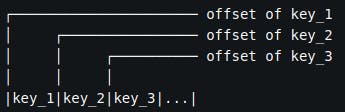
Figure 1. Key layout in memory
Where individual keys are encoded according to Figure 2.
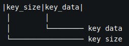
Figure 2. Single key encoding in memory
When we need to figure out if a certain key is in the set or not we need to loop over the byte array and compare keys to the one we’re querying for. If we reach a position where query_key < key,
we’re done. This is called linear search [12] and it’s not efficient. Access complexity of this algorithm is \(O(n)\). This structure has no space overhead.
As we can see from the printouts below, computations dominate the results whether or not data is cached.
$ ./test 2048 1 1000
key count: 2048
containers: 1
iterations: 1000

linear_search: 3770.58 ns/op, 0.04 L3 misses/op, 1.96 L1d misses/op, 44197.41 instr/op
linear_search: data size: 18432

 $ ./test 2048 1000 1
key count: 2048
containers: 1000
iterations: 1

linear_search: 4001.22 ns/op, 3.50 L3 misses/op, 150.66 L1d misses/op, 44240.77 instr/op
linear_search: data size: 18432
Simple Index
If we want to do better, we first need to realize that while the keys themselves can be long, we don’t need to index keys at full lengths but only unique prefixes. Figure 3. shows a simple example of unique prefixes for a set of keys.
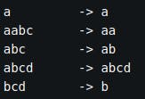
Figure 3. An example set of keys and their unique prefixes
Unique prefixes allow us to cut down on the index size and reduce the number of instructions we need for each comparison in it. We're building on top of the encoding shown in Figure 1 and Figure 2. Furthermore, we construct the index from every k-th entry’s unique prefix as shown in Figure 4 [**].
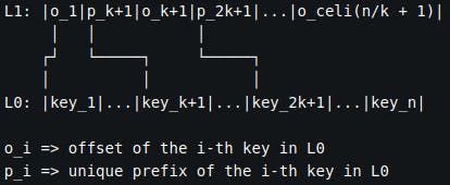
Figure 4. Memory layout for the simple index algorithm
With this structure, we’re splitting the set into buckets of size k. By doing this, we’ve effectively split the search area to \(n/k\) unique prefixes in the index plus the bucket the index pointed us to. Access complexity of this algorithm is \(O(n/k + k)\). Additional space that's required for the index is \(O(n/k)\).
Looking at the results below, we’ve managed to cut computations almost in half compared to the linear search above. It’s also way better in utilizing the cache which cuts the execution time more than 15 times.
$ ./test 2048 1 1000
key count: 2048
containers: 1
iterations: 1000

simple_index: 208.97 ns/op, 0.00 L3 misses/op, 0.24 L1d misses/op, 2194.17 instr/op
simple_index: bucket size: 32
simple_index: index size: 317
simple_index: data size: 18432

$ ./test 2048 1000 1
key count: 2048
containers: 1000
iterations: 1

simple_index: 275.95 ns/op, 1.27 L3 misses/op, 11.37 L1d misses/op, 2193.49 instr/op
simple_index: bucket size: 32
simple_index: index size: 317
simple_index: data size: 18432
[**] Index encoding in the framework is slightly different that what is shown in Figure 2, but functionally the same.
Binary Search
The way binary search works requires keys to be fixed in size. Since we’re working with variable length keys, we need to add a fixed-size index. We do this by simply encoding offsets for every key entry. Figure 5. shows the layout of the structure.
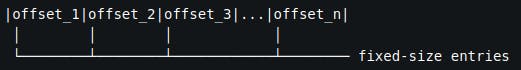
Figure 5. Memory layout for binary search algorithm
When the data is cached this algorithm performs better than all the others but falls short when that’s not the case. The issue lies in its access complexity which can be seen in the printouts below. It’s still faster than the simple index algorithm. Access complexity of this algorithm is \(O(log_2(n))\). Additional space required for the index is \(O(n).\)
$ ./test 2048 1 1000
key count: 2048
containers: 1
iterations: 1000

binary_search: 103.96 ns/op, 0.00 L3 misses/op, 0.29 L1d misses/op, 619.80 instr/op
binary_search: bsearch threshold: 4
binary_search: entries size: 4096
binary_search: data size: 18432

$ ./test 2048 1000 1
key count: 2048
containers: 1000
iterations: 1

binary_search: 236.77 ns/op, 3.62 L3 misses/op, 29.98 L1d misses/op, 606.93 instr/op
binary_search: bsearch threshold: 4
binary_search: entries size: 4096
binary_search: data size: 18432
One thing to take note of is the presence of bsearch threshold parameter. It instructs the binary search algorithm to switch to linear search once the threshold is reached. The reason for that is the fact that for really small sets linear search performs better despite having worse computational complexity [12]. This can be seen in the printout below [***].
$ ./test 4 1 100000
key count: 4
containers: 1
iterations: 100000

linear_search: 25.81 ns/op, 0.00 L3 misses/op, 0.00 L1d misses/op, 174.75 instr/op
linear_search: data size: 36

binary_search: 39.76 ns/op, 0.00 L3 misses/op, 0.00 L1d misses/op, 254.25 instr/op
binary_search: bsearch threshold: 1
binary_search: entries size: 8
binary_search: data size: 36
We can see here that the number of instructions executed for linear search is smaller, hence linear search performs better.
[***] For this printout bsearch_threshold template parameter was changed to 1.
Succinct prefix tree
As with the simple index algorithm, we’re going to split the input set into buckets of size k and we’ll be putting every k-th entry’s unique prefix with its offset in the index. Access complexity for this algorithm is \(O(m+k)\) where \(m\) is the maximum length of the unique prefixes. As we can see in the printout, the index is the smallest in the bunch. Additional space requirement is \(O(m).\)
$ ./test 2048 1 1000
key count: 2048
containers: 1
iterations: 1000

fst_index: 138.58 ns/op, 0.00 L3 misses/op, 0.28 L1d misses/op, 1793.65 instr/op
fst_index: bucket size: 32
fst_index: index size: 304
fst_index: data size: 18432

$ ./test 2048 1000 1
key count: 2048
containers: 1000
iterations: 1

fst_index: 206.71 ns/op, 1.28 L3 misses/op, 14.95 L1d misses/op, 1784.11 instr/op
fst_index: bucket size: 32
fst_index: index size: 304
fst_index: data size: 18432
B+ tree
To implement b+ trees for this, we can extend what we did in the simple index algorithm. We simply go through the index we created with simple index algorithm (L1), split it into buckets of size l and create a higher-level index containing \(n/(kl)\) entries (L2). We repeat this process until the highest level we create has no more than \(l\) entries (L3). We're building on top of the layout in Figure 3. The layout of the tree can be seen in Figure 6.
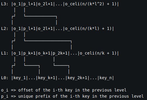
Figure 6. Memory layout for B+ tree algorithm
In essence, the only thing we’re doing is appending unique prefixes to the level’s data while keeping track of key counts and offsets. We emit every l-th unique prefix to the higher level. Access complexity of this algorithm is \(O(log_l(n/k) + k)\). Additional space required for the index is \(O(log_l(n/k))\).
Printouts show that using a b+ tree is even better than using a succinct prefix tree index. It has better memory access performance and executes in fewer instructions despite having a slightly bigger index.
$ ./test 2048 1 1000
key count: 2048
containers: 1
iterations: 1000

btree_index: 130.63 ns/op, 0.00 L3 misses/op, 0.22 L1d misses/op, 1221.82 instr/op
btree_index: elements per node: 8
btree_index: bucket size: 32
btree_index: index size: 362
btree_index: data size: 18432

$ ./test 2048 1000 1
key count: 2048
containers: 1000
iterations: 1

btree_index: 199.08 ns/op, 1.25 L3 misses/op, 12.59 L1d misses/op, 1208.54 instr/op
btree_index: elements per node: 8
btree_index: bucket size: 32
btree_index: index size: 362
btree_index: data size: 18432
Conclusion
A summary of running the test suite can be seen in the tables below. I've normalized results to the binary search algorithm since it performed best when data is cached and executes in the least number of instructions. Table 1. shows normalized results for the case when data is cached. L3 misses for this case were left out because they are close to zero for all algorithms. Table 2. shows normalized results for the case when the data is not cached.
| Algorithm | Time | L1d Misses | Instructions |
| Binary Search | 1.00 | 1.00 | 1.00 |
| Linear Search | 36.27 | 6.75 | 71.31 |
| Simple Index | 2.01 | 0.83 | 3.54 |
| Succinct Prefix Tree | 1.33 | 0.97 | 2.89 |
| B+ Tree | 1.27 | 0.76 | 1.97 |
Table 1. Relative algorithm performance when data is cached
| Algorithm | Time | L3 Misses | L1d Misses | Instructions |
| Binary Search | 1.00 | 1.00 | 1.00 | 1.00 |
| Linear Search | 16.90 | 0.97 | 5.03 | 72.89 |
| Simple Index | 1.17 | 0.35 | 0.38 | 3.61 |
| Succinct Prefix Tree | 0.87 | 0.35 | 0.50 | 2.94 |
| B+ Tree | 0.84 | 0.35 | 0.42 | 1.99 |
Table 2. Relative algorithm performance when data is not cached
Before all of this, I already had a full-blown B+ tree implementation [13] but it was somewhat complex and not all that efficient. This was a part of the reason I decided to look elsewhere. I wouldn’t have included B+ trees in this benchmark at all and would have been happy with the succinct prefix tree index but, while implementing the simple index algorithm, I realized that I can simplify the B+ tree implementation so I decided to include it after all.
This does confirm the assumption that from the CPU’s standpoint, all the memory layers are just progressively slower storage and that traditional techniques can still be used effectively on this scale.
Even though I didn’t end up using them, I’m glad I dug into succinct prefix trees because it gave me some other ideas on how to organize data on a larger scale but that’s a topic for another post.
References
[1] Wikipedia article on CPU cache: en.wikipedia.org/wiki/CPU_cache
[2] Latency Numbers Every Programmer Should Know: colin-scott.github.io/personal_website/rese..
[3] Wikipedia article on SDRAM: en.wikipedia.org/wiki/Synchronous_dynamic_r..
[4] Wikipedia article on Search algorithms: en.wikipedia.org/wiki/Search_algorithm
[5] Wikipedia article on B+ trees: en.wikipedia.org/wiki/B%2B_tree
[6] tyrdbs Database Toolkit Library: git.sr.ht/~tyrtech/tyrdbs
[7] Wikipedia article on LSM trees: en.wikipedia.org/wiki/Log-structured_merge-..
[8] Huanchen Zhang, Hyeontaek Lim, Viktor Leis, David G. Andersen, Michael Kaminsky, Kimberly Keeton, and Andrew Pavlo. 2018. SuRF: Practical Range Query Filtering with Fast Succinct Tries. In Proceedings of the 2018 International Conference on Management of Data (SIGMOD '18). Association for Computing Machinery, New York, NY, USA, 323–336.
[9] Blog post covering efficient select primitive implementation: pageup.hashnode.dev/on-the-path-for-a-bette..
[10] Indexing benchmark source code: git.sr.ht/~hrvoje/indexing-benchmark
[11] C++ standard library header: https://en.cppreference.com/w/cpp/header/random
[12] Wikipedia article on linear search: en.wikipedia.org/wiki/Linear_search
[13] Old tyrdbs' btree implementation source code: git.sr.ht/~tyrtech/tyrdbs/tree/14394d9fcf60..